Google ColabでPyTorch画像分類
こんにちは!うしじです。
先日、Google Colaboratoryでのファイル読み込み方法についての記事を書きました。
今回は、Google ColabでのPyTorchの画像分類を行います。 画像分類のプログラムは、Udacityのコースで開発したものをベースにしています。
ColabでのPyTorch利用
Google ColabでPyTorchを利用するのに、特にインストールは不要です。 Colab上で、下記を実行してみてください。インストール済みのPyTorchのバージョンが表示されます。 2020/5/24現在は、PyTorch v1.5.0 + CUDA 10.1 でしょうか。
In:
    import torch

    print(torch.__version__)

---
Out:
    1.5.0+cu101
開発するAI
今回は、PyTorchを用いて、画像分類AIを開発します。
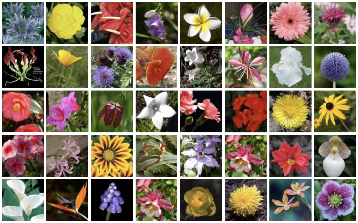
具体的には、花の写真から、その花が何なのかを推定するAIです。下記のような花の写真から、102種類の花の種類のうち、どれなのかを推定します。
利用するデータ
データには、102 Category Flower Datasetのものを使います。
test用、training用、validation用にデータを分けたものがここからダウンロード可能ですので、これを用います。
今回の画像分類では、
画像分類のステップ
下記のステップで進めています。
-
- 画像データのロードと前処理
-
- 画像分類AIのトレーニング
-
- トレーニング済みAIを用いた画像分類
画像分類のコード
ここから、Colab上の実際のコードを紹介していきたいと思います。
画像データのロードと前処理
まずは、必要なモジュールをImportします。
%matplotlib inline

import matplotlib.pyplot as plt
import numpy as np
import seaborn as sb

import torch
from torch import nn
from torch import optim
import torch.nn.functional as F
from torchvision import datasets, transforms, models

from PIL import Image

import json

from collections import OrderedDict
次に、画像ファイルを格納しているディレクトリを指定し、前処理を行います。
data_dir = '/content/drive/My Drive/Colab Data/flower_data'
train_dir = data_dir + '/train'
valid_dir = data_dir + '/valid'
test_dir = data_dir + '/test'


data_transforms = {
        'train' : transforms.Compose([transforms.RandomRotation(30),
                                       transforms.RandomResizedCrop(224),
                                       transforms.RandomHorizontalFlip(),
                                       transforms.ToTensor(),
                                       transforms.Normalize([0.485, 0.456, 0.406],
                                                            [0.229, 0.224, 0.225])
                                     ]),
        'valid' : transforms.Compose([transforms.Resize(256),
                                      transforms.CenterCrop(224),
                                      transforms.ToTensor(),
                                      transforms.Normalize([0.485, 0.456, 0.406],
                                                           [0.229, 0.224, 0.225])
                                     ]),
        'test' : transforms.Compose([transforms.Resize(256),
                                      transforms.CenterCrop(224),
                                      transforms.ToTensor(),
                                      transforms.Normalize([0.485, 0.456, 0.406],
                                                           [0.229, 0.224, 0.225])
                                    ])
}


image_datasets = {
        'train' : datasets.ImageFolder(train_dir, transform=data_transforms['train']),
        'valid' : datasets.ImageFolder(valid_dir, transform=data_transforms['valid']),
        'test' : datasets.ImageFolder(test_dir, transform=data_transforms['test'])
}


dataloaders = {
        'train' : torch.utils.data.DataLoader(image_datasets['train'], batch_size=64, shuffle=True),
        'valid' : torch.utils.data.DataLoader(image_datasets['valid'], batch_size=32),
        'test' : torch.utils.data.DataLoader(image_datasets['test'], batch_size=32)
}
また、データでは、花の種類を番号で表しているので、それを花の名前に紐付けるためのファイルの読み込みを行っておきます。
with open('/content/drive/My Drive/Colab Data/flower_data/cat_to_name.json', 'r') as f:
    cat_to_name = json.load(f)
ここまでで、画像データのロードと前処理は完了です。
画像分類AIのトレーニング
モデルやLearning rateを定義します。
今回の画像分類には、VGG-16を用いています。
また、Colabでは、無料でGPUを使うことができるので、その設定もしておきます。
model = models.vgg16(pretrained=True)


classifier = nn.Sequential(OrderedDict([
                          ('fc1', nn.Linear(25088, 4096)),
                          ('relu1', nn.ReLU()),
                          ('dropout1', nn.Dropout(0.2)),
                          ('fc2', nn.Linear(4096, 102)),
                          ('output', nn.LogSoftmax(dim=1))
                          ]))

model.classifier = classifier


criterion = nn.NLLLoss()
learn_rate = 0.001
optimizer = optim.Adam(model.classifier.parameters(), lr=learn_rate)


device = torch.device("cuda:0" if torch.cuda.is_available() else "cpu")
validation用の関数を定義しておきます。
モデルのトレーニング時に呼び出して、学習が進んでいるか確認するのに使います。
def validation(model, validloader, criterion):
    test_loss = 0
    accuracy = 0
    for inputs, labels in validloader:

        inputs, labels = inputs.to(device), labels.to(device)

        output = model.forward(inputs)
        test_loss += criterion(output, labels).item()

        ps = torch.exp(output)
        equality = (labels.data == ps.max(dim=1)[1])
        accuracy += equality.type(torch.FloatTensor).mean()

    return test_loss, accuracy
トレーニングを行います。今回は、4epoch分トレーニングしました。
epochs = 4
print_every = 20
steps = 0

model.to(device)

for e in range(epochs):
    running_loss = 0
    for ii, (inputs, labels) in enumerate(dataloaders['train']):
        steps += 1

        inputs, labels = inputs.to(device), labels.to(device)

        optimizer.zero_grad()

        outputs = model.forward(inputs)
        loss = criterion(outputs, labels)
        loss.backward()
        optimizer.step()

        running_loss += loss.item()

        if steps % print_every == 0:
            model.eval()
            with torch.no_grad():
                test_loss, accuracy = validation(model, dataloaders['valid'], criterion)

            print("Epoch: {}/{}.. ".format(e+1, epochs),
                  "Training Loss: {:.3f}.. ".format(running_loss/print_every),
                  "Valid Loss: {:.3f}.. ".format(test_loss/len(dataloaders['valid'])),
                  "Valid Accuracy: {:.3f}".format(accuracy/len(dataloaders['valid'])))

            running_loss = 0
            model.train()
トレーニングが完了したら、テストします。 テストの結果、87.9%の精度で分類可能でした。
model.eval()
with torch.no_grad():
    test_loss, accuracy = validation(model, dataloaders['test'], criterion)

print("Test Loss: {:.3f}.. ".format(test_loss/len(dataloaders['test'])),
      "Test Accuracy: {:.3f}".format(accuracy/len(dataloaders['test'])))
トレーニング済みAIを用いた画像分類
トレーニングしたAIを実際に使ってみましょう。使うために、いくつか関数を定義しておきます。
- process_image: 画像の前処理
- imshow: 前処理をもとに戻し、画像を表示
- predict: 推論の実行
- plot_solution: 推論を実行し、その結果を表示
def process_image(image):
    ''' Scales, crops, and normalizes a PIL image for a PyTorch model,
        returns an Numpy array
    '''
    img = Image.open(image)

    #Reseize
    if img.size[0] > img.size[1]:
        img_resize = img.resize((int(256 * img.size[0] / img.size[1]), 256))
    else:
        img_resize = img.resize((256, int(256 * img.size[1] / img.size[0])))

    #Crop
    left = img_resize.size[0]/2 - 224/2
    top = img_resize.size[1]/2 - 224/2
    right = img_resize.size[0]/2 + 224/2
    bottom = img_resize.size[1]/2 + 224/2
    area = (left, top, right, bottom)
    img_crop = img_resize.crop(area)

    #convert to np array
    np_image = np.array(img_crop)/255

    mean = np.array([0.485, 0.456, 0.406])
    std = np.array([0.229, 0.224, 0.225])
    img = (np_image - mean)/std

    #Reorder dimensions
    img = img.transpose((2, 0, 1))

    return img
def imshow(image, ax=None, title=None):
if ax is None:
fig, ax = plt.subplots()
if title:
plt.title(title)
# PyTorch tensors assume the color channel is the first dimension
# but matplotlib assumes is the third dimension
image = image.transpose((1, 2, 0))
# Undo preprocessing
mean = np.array([0.485, 0.456, 0.406])
std = np.array([0.229, 0.224, 0.225])
image = std * image + mean
# Image needs to be clipped between 0 and 1 or it looks like noise when displayed
image = np.clip(image, 0, 1)
ax.imshow(image)
return axdef predict(image_path, model, topk=5):
''' Predict the class (or classes) of an image using a trained deep learning model.
'''
img = process_image(image_path)
img_tensor = torch.from_numpy(img)
model.requires_grad = False
model.eval()
img_tensor = img_tensor.to(device)
model.to(device)
img = img_tensor.unsqueeze_(0).float()
output = model.forward(img)
ps = torch.exp(output)
probs, indices = ps.topk(topk)
probs = probs.data.cpu().numpy()[0]
indices = indices.cpu().numpy()[0]
idx_to_class = {i:c for c,i in model.class_to_idx.items()}
classes = [idx_to_class[i] for i in indices]
return probs, classesdef plot_solution(image_path, model):
# Set up plot
plt.figure(figsize = (6,10))
ax = plt.subplot(2,1,1)
#Get correct flower name for image title
flower_num = image_path.split('/')[7]
title = cat_to_name[flower_num]
img = process_image(image_path)
imshow(img, ax, title);
probs, classes = predict(image_path, model)
flower_name = [cat_to_name[i] for i in classes]
plt.subplot(2,1,2)
sb.barplot(x=probs, y=flower_name, color=sb.color_palette()[0]);
plt.show()これで完成です!
実際に使ってみると、下記のように表示されます。
正しく予測できてますね。
image_path = test_dir + '/28/image_05230.jpg'
plot_solution(image_path, model)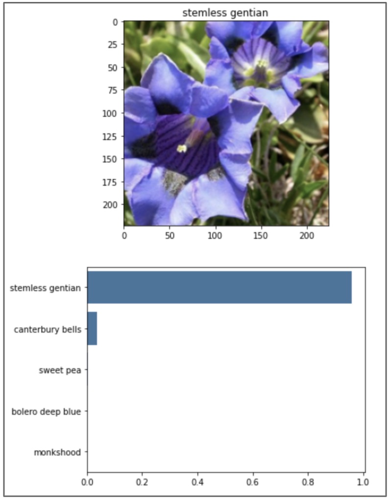
image_path = test_dir + '/2/image_05100.jpg'
plot_solution(image_path, model)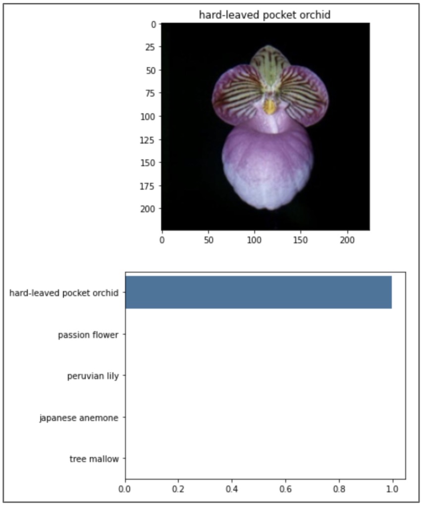
個人的には、TensorFlowより、PyTorchの方が好きです。
お勧めのPyTorchの書籍を紹介させていただきます。
